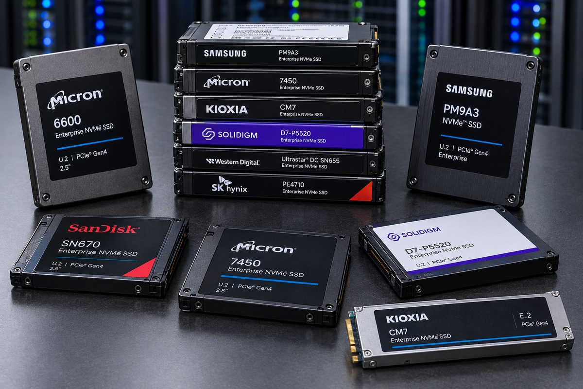
Deep expertise in solid-state storage systems: architectural modeling, NAND flash integration, host interface design, and performance validation. What that sentence actually means in practice — to design an SSD the full system must be understood. Modeling a drive allows the designer to test the designed performance, and measurements decide whether the design held.
An SSD is not a component. It is a small distributed system: a PCIe endpoint, a multi-core controller running a real-time firmware stack, a DRAM-resident index, an error-correction pipeline, a bank of independently-scheduled flash dies, and a power system that has to survive its own rail collapsing. Product design is the discipline of deciding how those pieces are sized against each other — before silicon exists, while the only thing available is a model.
A drive's spec sheet is the output of a model long before it is the output of a measurement. Performance validation is the process of finding out which one was wrong.
Architectural modeling
The drive as a chain of capacity-constrained stages. Which one is the limit, under which workload, in which time regime.
NAND integration
Cell type, die/plane parallelism, program-erase asymmetry, and the error mechanisms the ECC budget has to absorb.
Host interface design
PCIe and NVMe at the top, form factor and power envelope at the bottom.
Performance validation
Validating your modeling against real measurements.
01 — Architectural modelingThe drive is a min-cut problem
Every stage between the host and the media has a finite capacity. End-to-end performance is the smallest one.
A useful first-order model of an SSD treats the data path as a chain of stages, each with its own maximum throughput — the same shape as an arc capacity in a network-flow problem. Consider moving data as a shipping and receiving problem and you'll find many well documented models such as the capacity model (no, this is not the capacity of the drive). Data has to traverse every stage, so achievable performance is bounded by the narrowest link:
Within a stage, parallel resources add processing capacity: lanes, channels, dies, planes. Across stages, the pipeline moves only as fast as its minimum cut. The value of writing it this way is that it turns "is this drive fast?" into a specific, falsifiable question: which stage is the limit, for this workload, in this time regime?
The stages worth modeling
| Stage | First-order model | What makes it the limit |
|---|---|---|
| Host interface (PCIe) | N_lanes × LineRate × Encoding / 8 | Large-block sequential on a wide, fast media stack |
| Controller / FTL compute | N_cores × Clock / CyclesPerCommand | Small-block random IOPS, especially on DRAM-less parts |
| DRAM bandwidth | DataRate × Width / 8 × N_channels | Mapping-table traffic under random access |
| ECC / LDPC engine | CodewordSize × DecodeRate × N_engines | End of life, as retry and decode iterations climb |
| NAND channel bus | InterfaceClock × BusWidth × N_channels | A hard ceiling independent of array speed |
| NAND media / array | (PageSize × Planes × Dies × Channels) / t_op | The physical floor; t_op is t_R, t_PROG, or amortized t_BERS |
| pSLC write cache | burst vs. sustained computed separately | Sustained writes, once the cache is exhausted and folding starts |
| GC / write amplification | BW_host_sustainable = BW_media / WAF | Random writes on a full drive with thin over-provisioning |
| Queue depth (Little's Law) | IOPS_QD = QD / Latency_per_op | Shallow-queue workloads that can't fill the parallelism |
| Power / thermal | Peak_BW × DutyCycle(T, P_budget) | Sustained sequential in a small, poorly-cooled form factor |
Units have to match before you take the minimum. Some stages are naturally bandwidth-bound in GB/s, others operation-bound in IOPS. Converting through the workload's block size (BW = IOPS × block_size) is what determines which stages even compete: large-block sequential traffic tends to be won by the bandwidth-bound stages, small-block random by the IOPS-bound ones. The same drive has a different bottleneck at 4 KB random than at 128 KB sequential, and both numbers go on the datasheet.
The bottleneck is time-varying. A pseudo-SLC write cache means there are two different minima: a burst regime writing into cache at SLC program times, and a sustained regime once the cache is full and background folding to native TLC/QLC competes with host writes for the same channel and media bandwidth. Modeling only one of them produces a drive that benchmarks beautifully for ninety seconds.
02 — NAND flash integrationDesigning around an asymmetric medium
Pages are programmed and read. Blocks are erased. Nothing is overwritten in place. Everything else follows.
NAND stores bits as trapped charge in an array of charge-trap transistors wired in series — dense and cheap per bit, at the cost of only being usable in page and block granularities. The central asymmetry shapes the entire product: programs and reads happen at the page level, erases happen at the block level, and a page cannot be reprogrammed without an intervening block erase. See our discussion on the FTL and the parking garage analogy in the engineering notebook to gain a better understanding.
The basic NAND parameters drive much of the design limitations. Below is a list of some of the most important parameters.
| Operation | Granularity | Relative latency | Design consequence |
|---|---|---|---|
Read t_R | Page (~16 KB + spare) | tens of µs | Non-destructive; the fast path the whole QoS story is measured against |
Program t_PROG | Page | ~100s of µs – 2 ms | Density-dependent; SLC mode fastest, native QLC slowest |
Erase t_BERS | Block (~4–8 MB) | ~ms to 10+ ms | Amortized per page is what governs sustained throughput |
Density is a set of tradeoffs, not a number
Bits per cell is the primary product decision, and it is coupled to almost everything downstream. More voltage levels in the same cell means narrower margins between states, more sensitive sensing, faster wear per program/erase cycle, and a stronger ECC requirement:
| Type | Bits/cell | States | P/E endurance | Typical role |
|---|---|---|---|---|
| SLC | 1 | 2 | ~50k–100k | Write-cache tiers, industrial, pSLC regions |
| MLC | 2 | 4 | ~3k–10k | Legacy enterprise/prosumer |
| TLC | 3 | 8 | ~1k–3k | Mainstream client and enterprise today |
| QLC | 4 | 16 | ~100–1k | Capacity and read-heavy tiers |
| PLC | 5 | 32 | <100 | Cold/archival — still largely in development |
Current QLC parts require multi-pass programming, which often results in a drive requiring a pseudo-SLC mode as a write cache, then folding to native density in the background. That single decision is why burst and sustained write performance are different numbers, why the folding overhead has to be modeled as competing traffic, and why "what happens after the cache runs out" is the question that separates a datasheet from a product. However, the future is single-pass QLC programming, which is expected in products such as BiCS8–9.
Parallelism is the only real performance lever
The hierarchy — package → die → plane → block → page — is not organizational trivia. The die is the smallest independently-operable unit, with its own command queue, and it is the term that dominates both throughput and tail latency:
NAND read latency has barely moved in a decade. Drive-level read throughput has moved enormously. The difference is entirely die and channel count, plus an FTL that stripes addresses well enough to actually use them. Section 05 shows what happens when it doesn't.
The error mechanisms the design has to absorb
Raw bit error rate is not a defect — it is the operating condition. Read disturb accumulates errors in unread neighbors of heavily-read pages. Program disturb affects adjacent cells. Retention loss drifts the voltage distributions over time, faster when hot and faster near end of life. Cell-to-cell coupling gets worse with every added layer and every added bit per cell. Cumulative P/E wear raises the baseline across all of it.
The ECC engine exists to convert that noise back into data, and its capacity has to be budgeted against end-of-life RBER, not fresh-out-of-fab RBER. A decode engine sized for a new drive is a decode engine that becomes the binding stage in year four.
03 — The indirection layerThe FTL is the product
A flat L2P table, a garbage collector, and a durability scheme that survives losing power mid-write.
Hosts expect a flat, freely-rewritable LBA space. NAND cannot provide one. The flash translation layer resolves that mismatch by writing every update to a fresh pre-erased location and remembering where it went — and the structure that remembers is the logical-to-physical table.
See this writeup on the FTL in our engineering notebook. If you are new to the FTL, read the parking garage analogy.
In the enterprise case that table is flat, direct-mapped, and fully DRAM-resident: one entry per 4 KB LBA, indexed directly, sized at roughly 1 GB of DRAM per 1 TB of NAND. The payoff is that every address translation costs exactly one DRAM access regardless of access pattern — no secondary index, no cache miss, no extra NAND read just to find the mapping. That flatness is precisely why enterprise drives hold consistent random IOPS under sustained load where tiered, cached client schemes develop a latency tail of their own.
Write amplification is a consequence, not a bug
Because updates never land back on their old physical location, stale copies accumulate until garbage collection reclaims their blocks — relocating whatever is still valid first. That relocation is NAND traffic nobody asked for:
WAF ranges from roughly 1.05× on sequential or host-placement-managed traffic to 3–5× for worst-case random writes on a nearly-full drive. It divides sustainable write throughput directly, which is why over-provisioning, GC victim-selection policy, and workload sequentiality are all performance features, not housekeeping. GC hunts for the blocks with the least remaining valid data specifically because that is the cheapest space to reclaim.
Choosing a victim block efficiently needs a structure the L2P table can't provide — it answers "where does this LBA live," not "how much of this block is still current." So the FTL maintains a valid-page bitmap updated atomically with every mapping change, plus a compact per-block valid-page count that victim selection actually scans. Reverse lookup at relocation time comes from the LBA tag written into each page's out-of-band area, rather than a full physical-to-logical table that would double the DRAM bill and add a second structure to keep in sync. The greedy algorithm is one of the simplest and most commonly used for victim selection — look for a post on block selection in the future.
Surviving power loss
The table lives in volatile DRAM and changes on essentially every host write. Re-snapshotting it per write is a non-starter, so real designs layer three mechanisms:
- Checkpointing. The table is chunked, and only dirty chunks are flushed to NAND on a schedule — the same dirty-page-writeback idea an OS page cache uses. One final checkpoint is taken as the last act of an orderly power-loss shutdown.
- Journaling. Between checkpoints, individual mapping updates are appended to a small sequential log. Appending is cheap; touching the bulky table is not. Recovery loads the last valid checkpoint and replays the journal forward.
- Sequence numbers, and never overwriting the only copy. Every checkpoint and journal entry carries a monotonic generation number so recovery knows exactly what is newer than what. Checkpoints and the pointer identifying the current one are written to alternating slots, so a torn write leaves the previous intact copy as the fallback rather than corrupting the drive's record of itself.
Underneath all of it sits the backstop: every page's out-of-band area carries the LBA it holds. If the journal and checkpoint regions are both unusable, the FTL can rebuild the entire table by scanning the raw media. It takes minutes on a large drive, and it always works — which is why it earns its place in a design that should never have to reach for it.
04 — Host interface & form factorWhere the drive meets the platform
The protocol at the top, the power and thermal envelope at the bottom, and placement semantics in between.
Host interface design is usually discussed as PCIe generation and lane count, but that is the easy half. The harder half is that the form factor sets a power budget and a cooling method, and the power budget is what determines whether the drive can actually sustain the throughput the link and media can theoretically deliver. A deeper dive into current form factors can be found in the engineering notebook.
| Form factor | Cooling | Max power | PCIe | Role |
|---|---|---|---|---|
| U.2 (SFF-8639) | Passive, chassis airflow | ~9–25 W | Gen4/Gen5 x4 | Legacy-dominant enterprise; being displaced |
| U.3 (SFF-TA-1001) | Passive | ~9–25 W | Gen5 x4 | Tri-mode NVMe/SAS/SATA in one bay |
| E1.S | Passive → heatsink by thickness | ~20–25 W | Gen5 x4 (x8 opt.) | Hyperscale 1U mainstream; the M.2 successor |
| E1.L "ruler" | Passive / heat spreader | ~25–40 W | Gen5 x4/x8 | Capacity density; QLC cold/warm tiers |
| E3.S | Passive (1T) / heatsink (2T) | ~25–40 W | Gen5–Gen6, to x16 | Long-term U.2/U.3 replacement |
| E3.L | Heat spreader / heatsink | ~40–70 W | Gen5+, to x16 | Highest capacity; accelerator-capable chassis |
| M.2 22110 | Little or none integrated | ~4–11 W | Gen4/Gen5 x4 | Boot and cache drives; thermally constrained |
Note what these specs do not standardize: NAND package count, DRAM package count, and hold-up capacitor count are per-vendor PCB decisions constrained by available area, target capacity, and the required power-loss energy budget. That blank space in the spec is exactly where product design happens — and it is why a 15 mm U.2 and a 5.9 mm E1.S with the same controller are not the same product.
05 — Quality of serviceModeling the tail, not the average
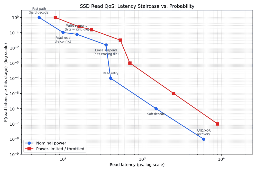
The centerpiece. Read latency QoS is a ladder of rare mechanisms, and each rung is both rarer and slower than the one before it.
Enterprise QoS specifications are written in percentiles — p99, p99.9, p99.99, sometimes p99.999 — and never in averages, for a structural reason: the mean is dominated by the fast path and barely moves when rare-but-slow events occur. A drive can post a beautiful ~50 µs average read latency and still fail its SLA because 1 read in 10,000 takes 2 ms.
The tail is not one phenomenon. It is a sequence of qualitatively different fallback mechanisms, each triggered only when the previous one is insufficient:
- Fast pathHard-decision decode succeeds first try, no contention. Baseline
t_R. - Read–read die conflictAnother read already in flight on the same die. ~2×.
- Write suspendThe read lands on a die mid-program; the controller suspends, services, resumes. ~3×.
- Erase suspendSame, but mid-erase — a coarser operation, so reaching a safe checkpoint costs more. ~7×.
- Read retryHard decode fails at the default reference voltage; re-read at shifted thresholds. ~5–10×.
- Soft decodeMultiple closely-spaced reads combined into per-bit LLRs for a soft-decision LDPC decode. ~20–50×.
- RAID/XOR (RAIN) recoveryReconstruct from the parity stripe: N−1 additional page reads plus XOR. ~100×+.
Die contention is a birthday problem
Treat each of QD outstanding reads as landing uniformly at random on one of N_dies dies — a reasonable first-order model when striping is good and access isn't pathologically hot-spotted:
This is the classic birthday setup — QD people, N_dies days — and conflicts appear faster than intuition suggests, because it only takes any pair colliding. On a 64-die drive (8 channels × 8 dies):
| QD | p = 1/N_dies | P(conflict on a die) | E[# contended dies] |
|---|---|---|---|
| 8 | 0.0156 | 0.64% | 0.41 |
| 16 | 0.0156 | 2.53% | 1.62 |
| 32 | 0.0156 | 8.90% | 5.70 |
| 64 | 0.0156 | 26.42% | 16.91 |
At QD32 on a 64-die drive, roughly one in eleven outstanding reads is waiting behind another operation on the same die. That is why deep queues trade average throughput for a fatter tail, and why the levers that fight it are more independent dies and better address striping — not faster NAND.
Ordinary write traffic is often the bigger contributor
A die can just as easily be mid-program or mid-erase when a read arrives. Modern NAND supports program-suspend and erase-suspend precisely so the read doesn't have to wait out a full t_PROG or t_BERS; it pays only the suspend/resume overhead. With uniform targeting, the hit rate is a simple ratio:
| Cause | Busy dies | P(hit) | Added latency |
|---|---|---|---|
| Write suspend | 4 of 64 | 6.25% | +100 µs |
| Erase suspend | 1 of 64 | 1.56% | +300 µs |
Worth sitting with: at these die counts a write-suspend hit (6.25%) is more common than a read–read conflict at QD16 (2.53%), and each one costs more. On a drive under real write and GC load, background write traffic can matter more to the tail than queue depth does.
The decode ladder
Every read returns noisy voltage-threshold data. Many LDPC engines escalate through four strategies, reaching for the next only when the current one fails:
| Stage | Extra NAND reads | Added latency | Trigger rate (healthy drive) |
|---|---|---|---|
| Hard decode | 0 | ~0, inline | dominant case |
| Read retry (voltage-shift search) | 1 to ~dozens | 10s–100s of µs | ~1e-4 – 1e-5 |
| Soft decode (LLR belief propagation) | several (3–7+) | 100s of µs – low ms | ~1e-6 – 1e-7 |
| RAID/XOR (RAIN) recovery | N−1 (stripe width) | single-digit ms | ~1e-8 – 1e-9 |
Reaching the last rung is not just slow — it is diagnostic. It signals a genuinely failing region and normally triggers wear-leveling and bad-block management, not merely a retry.
Power limiting shifts the whole distribution
Everything above is a rare-event mechanism: it fattens the tail while leaving the median almost untouched. Power and thermal limiting is categorically different. Under an NVMe power state, a slot power cap, or thermal throttling, the controller reduces effective parallelism — fewer dies and channels serviced concurrently, lower interface clock, scheduled idle windows. By Little's Law, the same arrival rate spread across fewer servers raises latency for the entire population, median included.
And the mechanisms compound rather than staying independent:
- Fewer active dies raises the binomial conflict rate. Keeping 32 of 64 dies active doubles
p, and conflict probability grows faster than linearly in that ratio. - Fewer active dies raises both suspend hit rates. The same absolute write and GC traffic now lands on a smaller pool — 6.25% / 1.56% becomes 12.5% / 3.13%.
- Higher temperature raises RBER. Retention loss accelerates with heat, so a throttled drive — hot by definition — pushes a larger fraction of reads into the decode ladder.
| Stage | Nominal — QD16, 64 dies | Power-limited — QD16, 32 dies |
|---|---|---|
| Fast-path latency | ~50 µs | ~80 µs |
| P(read–read conflict) | 2.5e-2 | 8.8e-2 |
| P(write suspend) | 6.25e-2 | 12.5e-2 |
| P(erase suspend) | 1.56e-2 | 3.13e-2 |
| P(read retry) | 1e-4 | 1e-3 |
| P(soft decode) | 1e-6 | 1e-5 |
| P(RAID/XOR recovery) | 1e-8 | 1e-7 |
The read–read conflict figure roughly triples while N_dies only halves — the binomial model is more sensitive to that ratio than linear scaling would suggest. Write and erase suspend, using the simpler ratio model, double exactly as expected.
Plotting it: the tail-latency staircase
Both axes have to be logarithmic. Latency spans ~50 µs to ~10 ms; probability spans 1 down to 1e-9. A linear probability axis would compress every rare-but-important event into an invisible sliver at zero, which defeats the purpose of the chart.
The y-axis is a proper tail probability — P(read latency ≥ this stage's latency), each stage's own probability plus every rarer and slower stage's. Plotting each stage's isolated probability instead would not decrease monotonically (write suspend at 6.25% is more probable than a read–read conflict at 2.53% despite costing more), and the curve would zig-zag for no physically meaningful reason. Treating the seven causes as mutually exclusive and exhaustive is a deliberate simplification — a read could in principle wait on a die conflict and then fail hard decode — but it keeps the plotted curve a well-behaved, monotonically non-increasing staircase.
The second chart isolates a single variable. Queue depth enters the model in exactly one place — the read–read conflict term — so holding power at nominal and sweeping QD across a fixed 128-die configuration moves one point and leaves the other six pinned:
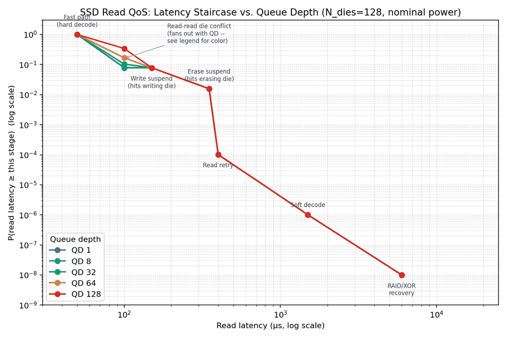
Both charts assume uniform random die targeting. Real workloads have locality — a sequential stream, a hot LBA range, or a small working set concentrates traffic onto fewer dies and makes conflict rates worse than predicted. Conversely, an FTL that tracks in-flight commands and actively steers new ones away from busy dies does better than pure random. The binomial number is a baseline for reasoning, not a guarantee. Knowing which direction a given workload pushes it is the actual skill.
06 — Performance validationMeasuring the thing you modeled
A QoS number measured under the wrong conditions is not a conservative estimate. It is a different number.
The practical conclusion from section 05 is uncomfortable for anyone quoting benchmark results: latency percentiles measured on an open bench with full airflow and no power cap do not describe the same drive in a power- or thermally-constrained enclosure. The envelope shifts the baseline and fattens the tail simultaneously. A meaningful QoS figure has to be measured — or at minimum modeled — inside the envelope the drive will actually ship in.
Validation that earns its name checks a few specific things:
- Steady state, not fresh-out-of-box. An unpreconditioned drive is measuring its pSLC cache. Sustained numbers require driving the drive into the regime where folding and GC are running.
- Both time regimes, reported separately. Burst and sustained have different binding stages. Averaging them describes neither.
- Percentiles to the depth the SLA specifies. Measuring p99 when the spec says p99.999 is three orders of magnitude of unsampled tail. The rungs that matter most are exactly the ones a short run will never hit.
- Under the real power and thermal envelope. Including, where relevant, the throttled case as its own reported condition rather than a footnote.
- Against the model, not just against the spec. The value of having built the min-cut model is that a measurement that disagrees with it points at something specific — a stage that isn't behaving like its formula, or an assumption (striping quality, WAF, duty cycle) that was wrong.
SNIA's Solid State Storage Performance Test Specification is the industry reference for percentile-based measurement methodology, and it exists precisely because ad-hoc benchmarking produces numbers that don't survive contact with a datacenter.
ClosingModeling is the Answer
Every section above is the same discipline applied at a different layer. Write down a model that makes a falsifiable prediction. Be explicit about the assumption that makes it tractable — uniform die targeting, mutually exclusive latency causes, a duty cycle standing in for a throttle curve. Then measure under conditions honest enough that a disagreement means something.
The min-cut model tells you which stage to spend money on. The binomial die-contention model tells you that the answer to a fat tail is more independent dies and better striping, not faster NAND. The compounding analysis tells you that a QoS number measured outside the drive's real power envelope is describing a different product. And the validation plan tells you which of those beliefs survived.
Architectural modeling, NAND flash integration, host interface design, and performance validation are not four skills. They are one loop, run at four scales.
Notes on the numbers
Latency and probability figures throughout are illustrative order-of-magnitude values chosen to make the mechanisms legible — they are not any specific drive's datasheet. Both figures are generated by a runnable model (qos_read_latency_model.py) rather than drawn by hand, so the regime parameters, die counts, and queue depths are editable and the curves regenerate accordingly. Layer-count and endurance figures reflect industry-typical ranges as of 2026 and should be cross-checked against a target device's datasheet for real analysis. The LDPC retry/soft-decode ladder, RAIN recovery, and program/erase-suspend behavior described here reflect widely-documented general controller design practice rather than any one vendor's implementation.